Let’s remind ourselves about the definition of variance:
\[ \text{Var}(X) = E[ (X - \mu)^2 ] \]
That is, it’s the expected difference squared between an random variable \(X\) and its mean, \(\mu\). This is Prob ’n Stats Day 1 stuff.
Obviously, in most situations we don’t actually know the parameters of our probability distribution. Instead we have some sample data \(X_1, \ldots, X_n\). With our sample population, we try to estimate the parameters of our PDF. The most obvious example is estimating \(\mu\):
\[ \overline{X} = \frac{1}{n} \sum_{i=1}^n X_i \]
I would also guess that the average person would estimate variance in more-or-less the same way
\[ s^2_n = \frac{1}{n} \sum_{i=1}^n (X_i - \overline{X})^2 \]
And that person (like me) might be shocked to learn that \(s^2_n\) (the uncorrected sample variance) is a biased estimator! It will, in fact, consistently underestimate the true variance of the population! Allow me to demonstrate…
# `samples` is 100000 rows of 50 columns, each drawn from a
# normal distribution with μ = 0 and σ^2 = 1.
#
# Each row is represents an experiment with 50 observations
samples = np.random.normal(0, 1, (50, 100000))
def uncorrected_variance(sample):
""" Given a sample populations, computes the uncorrected
sample variance:
s^2_n = (1 / n) Sum( (x_i - μ)^2 )
"""
n = sample.size
μ = sample.mean()
s = np.sum(np.vectorize(lambda xi: (xi - μ)**2)(sample)) / n
return ss_uncorrected = np.apply_along_axis(uncorrected_variance, 0, samples)def plot_variance_exp(variances, true_μ=1):
mean = variances.mean()
lbl = str.format("Mean: {0:.4f}\nBiase: {1:.4f}", mean, mean - true_μ)
pyplot.hist(variances, bins=25, alpha=0.5)
pyplot.axvline(mean, color='b', linestyle='dashed')
pyplot.text(x=1.5, y=10000, s=lbl)
return Noneplot_variance_exp(s_uncorrected)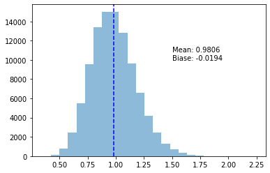
After running 100,000 experiments, being off by 2% sure seems like a lot! And again, it’s not just wrong, but consistently too small!
Correcting the Bias
Before we get to why \(s^2_n\) is biased, let’s actually start with the correction, and work backwards from there. As it happens, \(s^2_n\) will be off by a factor of \(\frac{n}{n - 1}\). This factor is known as Bessel’s correction (what a guy, Bessel…). Scaling up the uncorrected variance estimation by this factor gives us our corrected (and unbiased) variance estimator, \(s^2_{n-1}\).
\[ s^2_{n - 1} = \frac{n}{n - 1} s^2_n = \frac{1}{n -1} \sum_{i=1}^n (X_i - \overline{X})^2 \]
This new estimator is unbiased — I wouldn’t lie to you about that! But let’s run another experiment, just to make ourselves feel better.
def bessel_variance(sample):
    """Given a sample population, computes the corrected
    sample variance:

    s^2_(n-1) = (1 / (n - 1)) Sum( (x_i - μ)^2 )
    """
    n = sample.size
    μ = sample.mean()
    s = np.sum(np.vectorize(lambda xi: (xi - μ)**2)(sample)) / (n - 1)
    return s
s_corrected = np.apply_along_axis(bessel_variance, 0, samples)plot_variance_exp(s_corrected)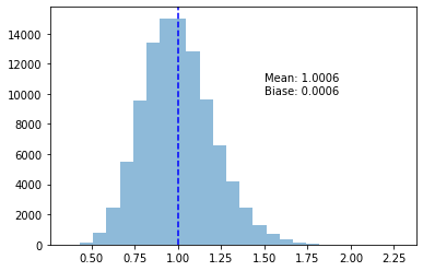
That’s more like it, huh! Now we’re seeing \(\overline{s^2_{n-1}}\) being within 0.01% of the true \(\text{Var}(X)\).
So… What Just Happened?
I have to admit, this kinda blew me away at first. I just happened to read somewhere “of course, the naive \(s^2_n\) estimator is biased”, and had to do a double take. I even pulled out my university Prob & Stats textbook to see if we learned this (as it happens, the book just defines \(s^2_{n-1}\), and says you should use that on the problem sets with no explanation…)
It is a very well known correction, though; I just seem to have missed the memo.
Luckily, though, it’s actually pretty simple to explain what went wrong with \(s^2_n\). To start, I’ll give a high-level explanation for the source of our bias.
High-Level Problem
There are two terms used to describe how “far-off” some \(X_i\) was from the “theoretical value”.
| Errors: | \(e_i = X_i - \mu\) |
| Residuals: | \(r_i = X_i - \overline{X}\) |
Often in experiments, the true \(\mu\) is unknown to us, and we are forced to estimate it with \(\overline{X}\). This means, in an experiment, we can measure the residuals but we may not be able to measure the errors.
Because \(\text{Var}(X) = E[ (X - \mu)^2 ]\), variance is the expected value of the sum of the squared errors. But we didn’t know the errors! We used the residuals instead. How well would things have worked if we knew the true errors, and not just the residuals?
def error_variance(sample):
    """ Given a sample populations, computes the sample variance with the
    known true μ, rather than the residuals. In our case, we know that μ=0.

    s^2_n = (1 / n) Sum( (x_i - μ)^2 )
    """
    n = sample.size
    μ = 0
    s = np.sum(np.vectorize(lambda xi: (xi - μ)**2)(sample)) / n
    return s
s_errors = np.apply_along_axis(error_variance, 0, samples)plot_variance_exp(s_errors)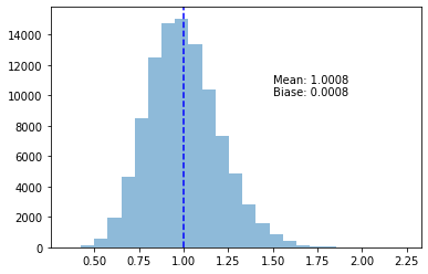
This, in fact, gives us an unbiased estimator! So obviously the secret lies in the difference between errors and residuals.
\(X_i - \mu\) and \(X_i - \overline{X}\) don’t seem that different, especially considering \(\overline{X}\) is an estimator for \(\mu\). As an estimator, though, \(\overline{X}\) is itself a random variable. The crux is that \(X_i\) and \(\overline{X}\) are not independent variables! A small part of \(X_i\) is “inside” \(\overline{X}\). So even though we are adding \(n\) terms together, we actually only have \(n-1\) degrees of freedom between those terms.
Put even more exactly, our uncorrected estimator is being drawn from a chi-squared distribution with only \(n-1\) degrees of freedom.
\[ \frac{1}{\sigma^2} \sum r_i^2 \sim \chi^2_{n-1} \]
But Where is the Bias Coming From?
Once we realize that the relationship between any \(X_i\) and \(\overline{X}\), we can quickly break things down and see where this bias is coming from. We’ve already noted that the true variance can be estimated as \(\frac{1}{n} \sum_i e_i^2\). We’re going to be using the residuals, however, which begs the question “what’s the relationship between \(e_i\) and \(r_i\)?”
\[ e_i = \underbrace{(X_i - \overline{X})}_{r_i} + (\overline{X} - \mu) \]
\[ \begin{align*} \frac{1}{n} \sum_i e_i^2 &= \frac{1}{n} \sum_i (r_i + (\overline{X} - \mu))^2\\ &= \frac{1}{n} \sum_i \left (r_i^2 + 2r_i(\overline{X} - \mu) + (\overline{X} - \mu)^2 \right )\\ &= \frac{1}{n} \left[ \sum_i \left( r_i^2 \right) + 2 \sum_i \left( r_i(\overline{X} - \mu) \right) + n(\overline{X} - \mu)^2 \right] \end{align*} \]
The first term is our “uncorrected estimator” (the mean of the residuals, rather than the errors). I want to dive into the middle term quickly, where we will see this interaction between \(X_i\) and \(\overline{X}\) play out.
\[ \begin{align*} \sum_i r_i(\overline{X} - \mu) &= \sum_i (X_i - \overline{X})(\overline{X} - \mu)\\ &= \sum_i \left( \overline{X}X_i - X_i\mu - \overline{X}^2 + \overline{X}\mu \right)\\ &= \overline{X} \sum X_i - \mu \sum X_i - n \overline{X}^2 + n\mu\overline{X}\\ \end{align*} \]
Now, of course \(\overline{X} = \frac{1}{n} \sum X_i\)…
\[ \begin{align*} &= n \overline{X}^2 - n\mu\overline{X} - n\overline{X}^2 + n\mu\overline{X}\\ &= 0 \end{align*} \]
Finally, we are left with a big fat bias staring back at us…
\[ \begin{align*} \frac{1}{n} \sum e_i &= \frac{1}{n} \sum r_i^2 + (\overline{X} - \mu)^2\\ &= s^2_n + (\overline{X} - \mu)^2 \end{align*} \]
How Does \(n - 1\) Fix This?
Well, we know that \(E\left[ \frac{1}{n} \sum e_i \right] = \sigma^2\), right? Then let’s take a look at the last line from above…
\[ \begin{align*} E\left[ \frac{1}{n} \sum e_i \right] &= E[s^2_n] + E[(\overline{X} - \mu)^2]\\ \sigma^2 &= E[s^2_n] + \frac{\sigma^2}{n}\\ E[s^2_n] &= \frac{n - 1}{n} \sigma^2 \end{align*} \]
And there it is! Simply scaling up by \(\frac{n}{n - 1}\) will yield an unbiased estimator!
So Always Use \(s^2_{n-1}\)?
That sure would make life simple, huh? Well I have bad news — the unbiased estimator will, in fact, yield a worse mean squared error. Here’s another simulation to demonstrate.
def MSE(estimates, θ=1):
    """Calculates the MSE of a set of estimates against a known θ."""
    n = estimates.size
    mse = np.sum(np.vectorize(lambda ti: (ti - θ)**2)(estimates)) / (n)
    return mse
mse_uncorrected, mse_corrected = MSE(s_uncorrected), MSE(s_corrected)
print("Uncorrected MSE: " + str(mse_uncorrected))
print("Corrected MSE: " + str(mse_corrected))
print("Percent Increase: " +
str(100 * (mse_corrected - mse_uncorrected) / mse_uncorrected))
> Uncorrected MSE: 0.039765490470560265
> Corrected MSE: 0.04101443329481074
> Percent Increase: 3.1407705763747864The MSE of Variance Estimators
A 4% increase in MSE… we just can’t win, can we!?
“So to minimize bias use \(s^2_{n-1}\), and to minimize error use \(s^2_n\)?”
My friend, meet \(s^2_{n+1}\)…
def mse_min_variance(sample):
    """Given a sample population, computes the sample variance,
    minimizing the MSE (for a normal distribution).

    s^2_(n+1) = (1 / (n + 1)) Sum( (x_i - μ)^2 )
    """
    n = sample.size
    μ = sample.mean()
    s = np.sum(np.vectorize(lambda xi: (xi - μ)**2)(sample)) / (n + 1)
    return s
s_mse_min = np.apply_along_axis(mse_min_variance, 0, samples)plot_variance_exp(s_mse_min)
MSE(s_mse_min)

>   0.03935094118106912
As it happens, for a normal distribution, \(s^2_{n + 1}\) will minimize our MSE. As is often the case in modeling and statistics, we have a trade-off to consider. Should we minimize the bias, or the MSE?
I should warn you, however, \(s^2_{n+1}\) will only minimize the MSE with a normal distribution. Different distributions will have their own optimal error-reducing estimators. Answering “why” is really a matter of crunching the numbers — I don’t think I can explain it better than Wikipedia does, but for completeness sake, let’s put the results here.
We can take a variance estimator \(s^2_a = \frac{1}{a} \sum (X_i - \overline{X})\), and calculate it’s MSE. This works out to (just trust me on this one):
\[ \text{MSE}(s^2_a) = \frac{n - 1}{na^2} ((n - 1) \gamma_2 + n^2 + n)\sigma^4 - 2 \left( \frac{n-1}{a} \right) \sigma^4 + \sigma^4 \]
A bit of a mouthful, but ok. \(\gamma_2\) here, by the way, is the excess kurtosis of this distribution (a measure of how “tailed” a distribution is). This is the kind of number that you could easily find for any distribution.
Now, to find the optimal \(s^2_a\) for some distribution, we simply minimize the MSE function, which happens when
\[ a = n + 1 + \frac{n - 1}{n} \gamma_2 \]
The normal distribution has \(\gamma_2 = 0\), which is where our \(a = n + 1\) is coming from. If we were drawing from a Bernoulli distribution, however, \(\gamma_2 = -2\), and we’d find \(a = n - 1 + \frac{2}{n}\).
That’s All, Folks!
It’s when the most mundane things don’t work as you’d expect that always seem the most exciting. I might be the last person to have gotten the memo on variance estimation. If not, though, I hope some of you were just as take by it as me.
Thanks for reading, and as always, leave a comment, and let me know your thoughts, questions, or comments!